
| |
Manual |
The SOMO (SOlution MOdeller) module of UltraScan (US-SOMO) initially contained only a bead modelling utility that was originally developed by the Rocco and Byron labs, respectively at the Istituto Nazionale per la Ricerca sul Cancro (IST, Genova, Italy) and at the University of Glasgow (Glasgow, Scotland, UK). The original code was mainly written by B. Spotorno, G. Tassara, N. Rai and M. Nollmann. The SoMo bead modeling utilities in SOMO are based on a reduced representation of a biomacromolecule, starting from its atomic coordinates (PDB format, mmCIF compatibility is still planned as of June 2024...), as a set of beads of different radii, from which the hydrodynamic properties in the rigid-body frame can be calculated, after overlaps between beads are removed, using the Garcia de la Torre-Bloomfield "supermatrix inversion" (SMI) approach (García de la Torre and Bloomfield, Q. Rev. Biophys. 14:81-139, 1981). The reduced representation is afforded by grouping together atoms and substituting them with a bead of the same volume, appropriately positioned. Importantly, the volume of the water of hydration theoretically bound to each group of atoms can be then added to each bead. The overlaps between the beads are then removed in sequential steps, but preserving as much as possible the original surface envelope of the bead model. The method was fully validated and reported in the literature (Rai et al., Structure 13:723-734, 2005; Brookes et al., Eur. Biophys. J., 39:423-435, 2010; Brookes et al., Macromol. Biosci. 10:746-753, 2010). Among the main advantages of this method over shell-modelling and grid-based procedures are a better treatment of the hydration water and the preservation of a direct correspondence between beads and original residues. For instance, the latter feature could be used to include flexibility effects into the computations. Furthermore, by identifying and excluding from the hydrodynamic computations beads that are buried and thus not "in contact" with the solvent, a large span in the size of the structures that can be analysed with this method without loss of precision is obtained: originally, structures from 5K to 450K were successfully studied, and the steady increase in the available computer power is continuosly expanding this range .
Subsequently, we have also improved the original AtoB grid method (Byron, Biophys. J. 72:408-415, 1997), which was already included within US-SOMO, by adding the theoretical hydration, accessible surface area screening, and a better preservation of the original surface. The possibility of changing the grid size in the improved AtoB could be very useful to study very large structures and complexes.
Later on, in US-SOMO was added an alternative, at the time far more computationally intensive method of calculating the hydrodynamics based on the analogy that exists between certain hydrodynamic and electrostatic properties, ZENO (see Douglas, Some Applications of Fractional Calculus to Polymer Science, Adv. Chem. Phys. 102:121-191, 1997; Douglas et al., Hydrodynamic friction and the capacitance of arbitrarily shaped objects, Phys. Rev. E 49:5319-5331, 1994; Mansfield et al., Intrinsic Viscosity and the Electric Polarizability of Arbitrarily Shaped Objects, Phys. Rev. E, 64:61401-61416, 2001; https://zeno.nist.gov/). Then, in May 2014 an interface and an analysis modulus for the boundary elements method BEST [S.R. Aragon, A precise boundary element method for macromolecular transport properties. J. Comp.Chem., 25, 1191-1205 (2004); S.R. Aragon and D.K. Hahn, Precise boundary element computation of proteins transport properties: Diffusion tensors, specific volume and hydration, Biophysical Journal, 91:1591-1603, 2006] were implemented within US-SOMO.
In 2015, a comprehensive study was conducted to compare various hydrodynamic modeling approaches (Rocco and Byron, Computing translational diffusion and sedimentation coefficients: an evaluation of experimental data and programs., Eur. Biophys. J. 44:417-431, 2015, Erratum http://dx.doi.org/10.1007/s00249-015-1058-1; see also Rocco and Byron, Hydrodynamic Modeling and Its Application in AUC, Methods Enzymol. 562:81-108, 2015). The methods tested were SoMo with computations using either the SMI or ZENO approaches, AtoB with 5 and 2 Å grid sizes and SMI computations, BEST, all under the US-SOMO implementation, and, externally, HYDROPRO (Ortega, A., D. Amorós, and J. García de la Torre. Prediction of hydrodynamic and other solution properties of rigid proteins from atomic- and residue-level models. Biophys. J. 101:892-898, 2011). The results indicated that, on average, BEST and HYDROPRO tend to underestimate the translational frictional properties by ~-3 and -4%, respectively, while SoMo using either the SMI or ZENO approaches overestimates them slightly less (~+2%). The best results using the SMI approach were obtained by AtoB with a 5 Å grid size, ~+0.5. However, a combination of SoMo bead models without overlap removal and ZENO computations performed even better, with ~0% average discrepancy and all results within ±4%, not far from the average experimental error of ±~3%. For these reasons, starting from the May 2015 US-SOMO release, this combination was directly offered among the bead modeling hydrodynamic computations options.
In 2017, a new implementation of the ZENO method, completely rewritten in the C++ language instead of Fortran, with greatly improved serial performance and able to utilize the multi-core capabilities of modern processors, thus allowing computational times shorter by a factor of ~100, was produced at NIST (Juba et al., J. Res. Natl. Inst. Stand. Technol. 122:1-2, 2017). This new ZENO code was implemented into US-SOMO, but it could be distributed only with Linux system executables. This was due to the US-SOMO underlying architecture which relied on the Qt3 now obsolete libraries. A major rewriting effort was then done, to recode US-SOMO under the up-to-date Qt5 framework. This has allowed us to introduce a new bead model generating option, which we call "van der Waals (vdW) with overlaps". The vdW with overlaps method allows generating a bead model where each atom present in the PDB file (except, by default, H2O molecules) is represented by a bead whose radius is equal to the atom's van der Waals radius as listed in the somo.residue table (see below). If water molecules are associated to any particular atom in the somo.residue table, their volume is calculated and added to that derived from the atom's van der Waals radius, and a final bead radius is then recomputed. No overlap removal is performed, and the ZENO method could then be used to compute the hydrodynamic parameters. While this direct method originally matched slightly worse the experimental parameters of the test proteins (Brookes and Rocco, Recent advances in the UltraScan SOlution MOdeller (US-SOMO) hydrodynamic and small-angle scattering data analysis and simulation suite. Eur. Biophys. J. 47:855-864, 2018), it opens up some interesting possibilities, such as using structures explicitly hydrated by Molecular Dynamics simulations. The vdW with overlaps method is under active development, and new features bringing its performance on par and even better than those described in the above-mentioned paper have been added for the July 2024 release (Brookes and Rocco, manuscript in preparation).
In 2018, a new computational method that could handle bead models with overlapping beads of different size has been presented (Zuk et al., GRPY: an accurate bead method for calculation of hydrodynamic properties of rigid biomacromolecules, Biophys. J. 115:782-800, 2018). GRPY (Generalized Rotne-Prager-Yamakawa) works in the same framework as the SMI method, while solving the long-standing issue of overlaps between beads of different sizes and providing robust estimates of the intrinsic viscosity and the rotational diffusion coefficients (the latter are not computed by ZENO), but is rather more computationally intensive. A non-parallel GRPY code was made available within US-SOMO as an additional computational option, and a full implementation allowing multi-core parallel processing is now available for all operating systems from the July 2024 release.
Importantly, the GRPY availability has allowed us to re-examine the performance of the SMI method for what concerns models with non-overlapping beads. While small differences were found for the translational diffusion properties computations, we are sorry to report that the SMI calculations of the rotational diffusion and the intrinsic viscosity did not match the state-of-the-art GRPY results for simple bead models (linear arrays, compact arrays, round arrays, all with equal radius) test structures, with up to 40% differences for the rotational diffusion properties. This failure directly stems from the inadequacy of the so-called "volume correction" that was originally developed by J. García de la Torre and collaborators and that is implemented in the SMI routines (see Spotorno et al., Eur. Biophys. J. 25:373-384, 1997; Erratum 26:417, 1997). While the García de la Torre group has subsequently introduced improvements for the computation of the rotational diffusion and the intrinsic viscosity (see García de la Torre et al., Improved calculation of rotational diffusion and intrinsic viscosity of bead models for macromolecules and nanoparticles. J. Phys. Chem. B 111, 955-961, 2007), it turns out that these can be applied only for non-overlapping beads of equal size. Therefore, from the February 2021 US-SOMO release, the SMI method hydrodynamic computations output will NOT report anymore the rotational diffusion properties and the intrinsic viscosity values. Users interested in these calculations can utilize the state-of-the-art GRPY method, that is, however, computationally demanding, or, limited to the intrinsic viscosity calculation, the ZENO method, that can handle large structures.
Importantly, the availability of parallel GRPY and the vdW models has allowed us to test in detail the performance of the ZENO method. We found that the ZENO calculation of Dt(20,w) constantly produced relatively larger (~+1-2%) values than those computed by GRPY for our test set of 25 protein structures. We could track a dependency on the "skin thickness" parameter in the ZENO calculations, that correlated linearly, although not perfectly, with the radius of gyration Rg of those proteins. Surface roughness appeared also to be a factor, but calculations of a proxy for this feature, the mass or surface fractal dimensions (Dm and Ds) did not produce any useful correlation. Incidentally, stemming from this work the calculations of Dm and Ds can now be performed as an option on loading a (bio)-macromolecular structure in US-SOMO. Using more elongated structures (derived from the fibrinogen main body crystal structure 3GHG.pdb) we found that the ZENO skin-dependence of the differences with the GRPY calculations reached a plateau at Rg values of 50-60 Å. The Rg-dependence of this entire dataset of 33 protein structures was fitted with a sigmoid, and using this skin thickness heuristic dependence reduced the discrepancy between GRPY and ZENO calculated Dt(20,w) values to an average of 0.5±0.22% (range ±0.6%) (Brookes and Rocco, manuscript in preparation). This heuristic ZENO skin value calculation is now offered as a default option from the July 2024 release of US-SOMO.
US-SOMO also includes a fully functional Small-Angle X-ray or Neutron Scattering (SAXS/SANS) simulator module, which works on either the original atomic structure, or on a bead model, and has enhanced experimental data processing capabilities. In the modeling area, several methods are offered for the computation of SAXS and SANS I(q) vs. q curves. Some of these methods require explicit hydration of the PDB structure(s), which should be presently externally provided. A pairwise-distance distribution function P(r) vs. r computation starting from a PDB structure is fully operational for both SAXS and SANS, and includes a graphical mapping utility to visualize which residues in the structure are contributing to specified distance ranges. An indirect Fourier transform Bayesian algorithm, based on the work by Hansen (Hansen, J. Appl. Crystallogr. 33:1415-1421, 2000; Hansen, J. Appl. Crystallogr. 41:436-445, 2008), has been implemented for the computation of the pairwise distance distribution function from SAS data.
In the experimental data processing area, a novel HPLC-SAXS data
processing utility has been implemented, which starts with the transformation of a time series of I(q) vs.
q frames into a series of time chromatograms I(t) vs. t for each q value. A check of the baselines, potentially revealing capillary fouling due to the accumulation of material on its walls, can then be performed, and corrections applied. In case of overlapping or not baseline-resolved peaks, Single Value Decomposition (SVD) can be applied on the original or baseline-corrected data, the latter after automatic back-generation of the I(q) vs. q frames, to identify how many components are present in the data. Global Gaussian analysis/decomposition can then be performed on the I(t) vs. t for each q value dataset, followed by back-generation of the I(q) vs. q frames for each Gaussian peak. Several improvements are present in this area from the June 2015 release, like an integral baseline evaluation/subtraction procedure, with immediate testing of the results in the I(q) vs. q space, the possibility of peak decomposition using non-symmetrical Gaussian functions, an improved treatment of concentration detector data, and a tool to evaluate the data-associated errors, when necessary, from the baseline fluctuations.
The Guinier analysis of experimental I(q) vs. q curves offers the determination of the overall z-average square radius of gyration <Rg2>z and of the w-average molecular weight <M>w from global Guinier, of the z-average square cross-section radius of gyration <Rc2>z and of the w/z-average mass per unit length <M/L>w for rod-like macromolecules, and of the z-average square transverse radius of gyration <Rt2>z and of the w/z-average mass per unit area <M/A>w for disk-like marcomolecules.
From the July 2024 US-SOMO release, modules to analyse Multi-Angle Light Scattering (MALS) data and integrate them with in-parallel or sequentially collected SAXS data have been added.
The batch operations module includes supercomputing access, with an interface to Discrete Molecular Dynamics (DMD) programs (Dokholyan, NV, Buldyrev, SV, Stanley, HE, and EI Shaknovich. Discrete molecular dynamics studies of the folding of a protein-like model. (1998) Folding & Design 3:577-587; Ding F, Dokholyan NV. Emergence of protein fold families through rational design. Public Library of Science Comput Biol. (2006) 2(7):e85). Starting from the May 2014 release, you will also find the implementation on a supercompute cluster of the boundary-elements hydrodynamic computations BEST [S.R. Aragon, A precise boundary element method for macromolecular transport properties. J. Comp.Chem., 25, 1191-1205 (2004); S.R. Aragon and D.K. Hahn, Precise boundary element computation of proteins transport properties: Diffusion tensors, specific volume and hydration, Biophysical Journal, 91:1591-1603 (2006)], and the relative interfaces in US-SOMO to set-up the analysis parameters and analyze the computations results.
Other features include a model classifier in which calculated parameters can be compared and ranked against experimental data, and a PDB editor.
The program main window contains an upper bar from which all the options governing its operations can be controlled, and a main panel for program execution. However, due to its high level of sophistication, properly setting all the available options can be non-trivial for the general user. Therefore, the US-SOMO module is distributed with pre-defined default options that should allow the direct conversion of a PDB-formatted biomacromolecular structure file into a bead model, and the computation of its hydrodynamic properties, without the need of accessing the advanced options menus. In particular, the workhorse SoMo approach, either with or without overlaps removal (the latter now being the preferred option since the ZENO and GRPY implementation) is based on properly defining the atoms and residues found in PDB files, and the rules allowing their conversion into beads. These rules also apply for the vdW bead models. The US-SOMO distribution includes the definition of all the standard amino acids, nucleotides, carbohydrates, and common prosthetic groups and co-factors, but this list is by no means exhaustive, and the need to code for "new" residues is not a remote possibility. As this operation can be demanding, notwithstanding the user-friendly GUIs governing it, the pre-defined set of options includes approximate methods to deal with either missing atoms within coded residues, and/or not yet coded residues. Starting from the May 2015 release, the default option for SoMo models is to generate a single bead for each non-coded residue using average parameters. When non-coded residues are found, a pop-up panel will alert the user and present as options (i) to continue with the approximate method; (ii) to skip non-coded residues (not recommended), or (iii) to halt operations and then take proper action like coding for the new residue. For coded residues with missing atoms, since most often this is due to lack of crystallographic data, the SoMo bead modeling method default option is now to use the complete residue's bead(s), appropriately positioned (again, a pop-up panel will warn of such instances and present the alternative skip (not recommended) or halt operations options). Obviously, there's no cure for completely missing residues, which will have to be built in the original structure for reliable results, since the structure should contain all residues and atoms that are present in the "real" macromolecule studied in solution. This applies also for missing atoms if vdW models are to be used. Therefore, for best performance all residues should be properly coded in the US-SOMO tables (see below).
 |
SOMO Program:
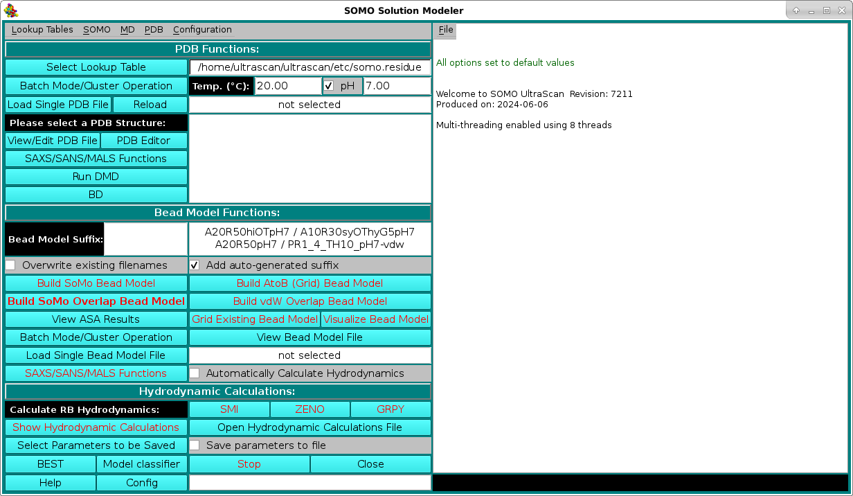
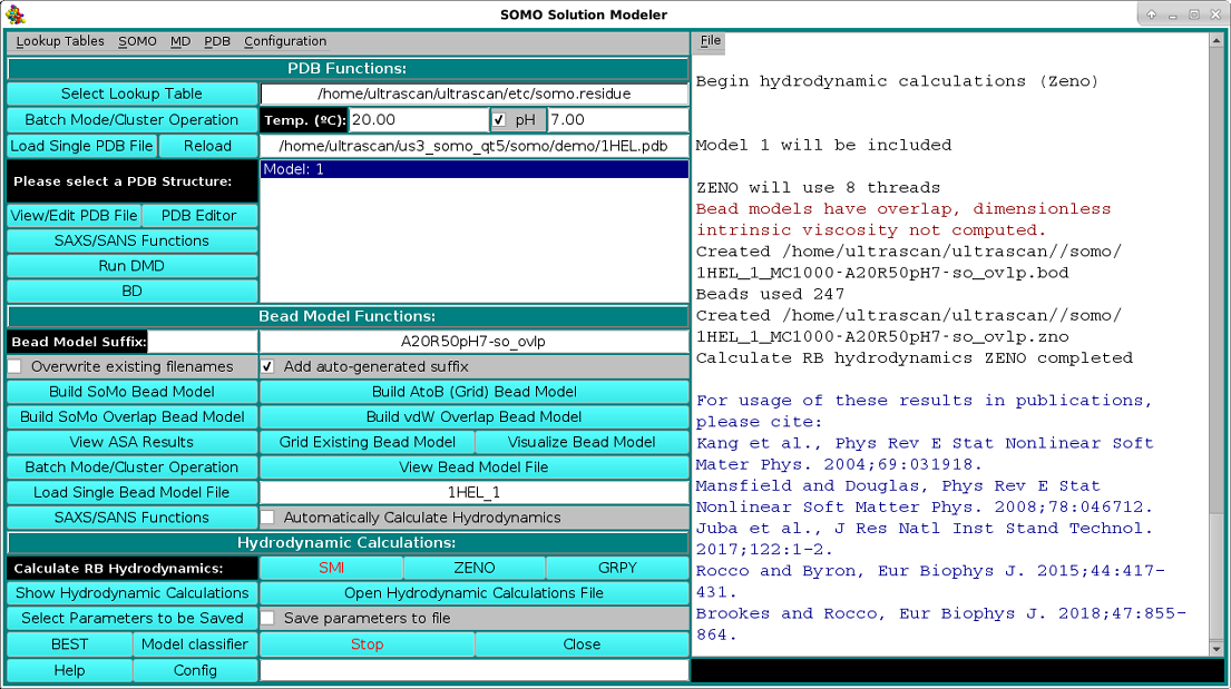
These functions control the execution of the US-SOMO program, whose progress is recorded in the right-side main window (in the pictures that follow below, excerpts of the messages during the model building and hydrodynamic computation phases starting from the 1HEL.pdb hen white lysozyme structure will be shown). They are divided in three subpanels controlling operations that deal with the primary PDB file (PDB Functions:), operations relating the generation of bead models (Bead Model Functions:), and the computation of the hydrodynamic parameters (Hydrodynamic Calculations:). Note that the buttons that can be actuated at a given stage of operations are identified with black labels, while not-actuable buttons are identified with red labels. This color scheme can be changed from the System Configuration menu accessisble form the Configuration pull-down menu in the top bar.
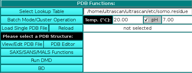 |
PDB Functions:
On launching, US-SOMO will automatically load the last used lookup table (default: somo.residue), where all the informations needed to convert the residues present in atomic structures into beads are stored. To select a different lookup table, click on Select Lookup Table. You can create multiple
lookup tables for different conditions. The lookup table needs to contain all atoms and residues present in the (macro)molecule to be loaded in the next step. By default, US-SOMO will automatically load the last used *.residue table.
A new feature available since the February 2021 release is the presence of two additional fields for the temperature T (default: 20 °C) and the pH (default: 7.00; if this number is modified, rechecking the checkbox associated with this entry will restore the default value) at which some calculations are then performed (see below) and some properties are defined. In particular, the pH controls the ionization state of atoms that can either gain or loose a proton, such as the NH2 amino group or one of the oxygens in the COOH carboxy group. This in turn affects the molecular weight and the hydration of the residue, and for this reason new fields were added in the somo.residue table allowing to enter the pKa of an atom and the hydration values at the pH extremes of 0 and 14 (see here). For a chosen pH, the Henderson-Hasselbalch Equation (see Po and Senoza, J. Chem. Educ. 78:1499-1503, 2001) is used to find the relative proportions of protonated/deprotonated species for each ionizable atom for which a pKa is defined within a residue (for polyprotic species a system of Henderson-Hasselbalch equations is solved). Basically, for the dissociation of an acid HA into A- and a proton you have:
log10 [A-]/[HA] = pH - pKa
[A-]/[HA] = 10(pH-pKa)
If one considers [A-] = I , the ionized fraction, then [HA] = 1 - I is the non-ionized fraction. Therefore:
10(pH-pKa) = I/(1-I)
In this way, we can calculate the fraction of protons bound to each ionizable atom and the fraction of hydration waters associated with it as a function of the entered pH. From the proton counts, summation over the entire protein allows to calculate the overall anhydrous Molecular Weight and the net charge at the entered pH. The Henderson-Hasselbach equation is also used in an iterative way over all ionizable atoms to find the isoelectric point of the (bio)macromolecule under examination. These values are now reported in the progress window after loading a PDB structure.
As for T, note that by default the hydrodynamic calculations are always performed at "standard conditions" (water at 20 °C), irrespective of the T value set here. However, temperature and buffer conditions can by changed in the Hydrodynamic Calculations Options) module.
Two alternative options are available to load an atomic structure, such as those derived from NMR, X-ray crystallography, or cryo-EM data, the Batch Mode Operation (see here), or the standard Load Single PDB File. Selecting a PBD file will also automatically call the molecular visualization program RasMol (Sayle RA, Milner-White EJ. RasMol: biomolecular graphics for all. Trends Biochem. Sci. 20:374-376, 1995) which will display the structure(s) in a pop-up window. For Linux-based systems, RasMol needs to be installed in
$ULTRASCAN/binfor 32 bit machines, and
$ULTRASCAN/bin64for 64 bit platforms. You can get a copy of RasMol from http://www.bernstein-plus-sons.com/software/rasmol/ (recommended, there it's under active development), or from http://www.umass.edu/microbio/rasmol/, or from http://openrasmol.org/#Software.
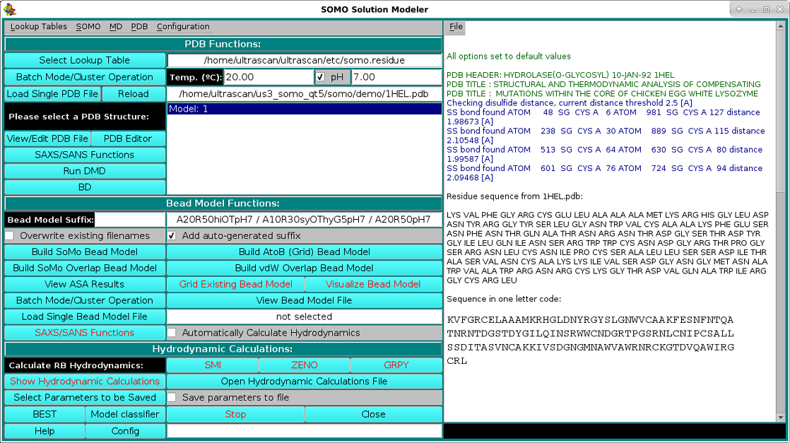 |
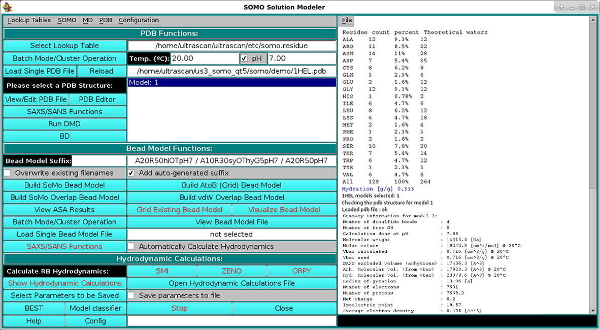
As shown in the picture above, besides visualizing the structure, the HEADER and TITLE fields of the PDB file will be displayed in the progress window, followed by a list of identified disulfide bonds between CYS residues, if any. This is a feature that was already present but was never made operational until the February 2021 release. It's active now by default, but can be turned off from the PDB parsing pull-down menu, where the cut-off distance (default: 2.5 Å) can also be changed. Importantly, if unpaired CYS residues are identified, their name will be changed to "CYH", for which a special entry is defined in the somo.residue table, since some molecular properties slightly differ between free cysteines and disulfide-bonded cystines. The residues sequence in both three- and one-letter codes (both "CYS" and "CYH" are reported as "C" in the latter) is then displayed, followed, as shown in the picture below, by a summary of each reside count, percentage, and its associated, pH-dependent theoretical waters of hydration and the corresponding global hydration (g/g, i.e. g water/g protein), and by a list of various molecular properties calculated for the model: number of disulfide bonds, number of free SH, molecular weight, molar volume, partial specific volume (vbar) calculated at the specified T and the one that will be used in the hydrodynamic calculations, anhydrous SAXS excluded volume, anhydrous and hydrated molecular volumes computed from vbar and the global hydration (using the water molecular volume as defined in the Miscellaneous Options panel), number of electrons, number of protons (pH-dependent), net charge at the specified pH, isoelectric point, and the average electron density:
 |
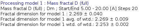
Note: from the July 2024 US-SOMO release, if the calculation of the Fractal Dimension has been enabled from the Fractal Dimension Options in the SOMO list of pull-down menus (see here), the results will be shown after the other parameters in the main progress window, as in the image below for the mass fractal dimension Dm calculations:
 |
This option is fully described here.
If problems are encountered with the selected PDB file, like the presence of non-coded residues or missing atoms within coded residues, they will be reported in the progress window either as warnings or errors. Starting from the May 2015 release, if non-coded residues or coded residues with missing atoms are found,
a pop-up panel will appear warning of the occurence and offering the alternative options to continue using approximate methods, skip the whole residue, or stop the program execution, waiting for corrective action to be taken.
The original PDB file can be viewed and, if necessary, edited by clicking on the View/Edit PDB File
button. In addition, we have developed and made available an advanced PDB editor (see
here).
The PDB file can contain multiple models and if so, multiple models will be displayed by
RasMol and in the list box. In this case, you can select just a single model,
or multiple models by holding the crtl key while clicking on the models' names (crtl-A selects
all models). If multiple models are selected, all subsequent operations (except the SAXS/SANS options)
are carried out sequentially on the selected models.
To allow for a quick re-calculation of molecular properties after changing T or pH, a new Reload button is now present next to the Load Single PDB File button. On pressing it, the last used PDB file will be reloaded.
Pressing the SAXS/SANS/MALS Functions button will take you to the SAXS/SANS/MALS module, where you can perform simulations on the selected PDB structure, or deal with experimental and/or previously generated data (see here). The SAXS/SANS/MALS module is in an advanced state but still under constant development (as of June 2024).
Pressing the RUN DMD button will first open the set-up panel for running a Discrete Molecular Dynamics (DMD) simulation on the selected structure. Once the parameters have been set, the DMD run can be launched through the Cluster utility of the Batch Mode/Cluster Operation module. The BD button, still not yet available in this release (July 2024), will allow running a Brownian dynamics simulation.
 |
Bead Model Functions:
Once a model structure (or multiple model structures in the case of NMR-style formatted data) are selected, the Build SoMo Bead Model,
Build AtoB (Grid) Bead Model, Build SoMo Overlap Bead Model, and Build vdW Overlap Bead Model buttons will also become active, offering alternative ways of generating a bead model. In particular, the third option, which will generate a SoMo-type bead model with overlaps without then removing them, is an addition made available starting from the May 2015 release, reflecting the conclusions of an extensive examination of all the hydrodynamic modeling/computational methods then available (Rocco and Byron, Eur. Biophys. J. 44:417-431, 2015). The fourth option, still under active development, has been added with the January 2018 release, and allows generating a bead model where each atom present in the PDB file is represented by a bead whose radius is equal to the atom's van der Waals radius as listed in the somo.residue table. If water molecules are associated to any particulat atom in the somo.residue table, their volume is taken into account in the definition of the bead's radius. As of July 2024, tests with an extended set of proteins have provided evidence that the vdW with Ovelaps models can now reproduce accurately their translational diffusion, rotational diffusion, and intrinsic viscosity parameters, although the exact details of the hydrated beads positioning are still under evaluation (Brookes and Rocco, manuscript in preparation). Note that if the latter two bead modeling methods are chosen, the SMI method will not be available, and only the ZENO and GRPY computational methods could be used (see below).
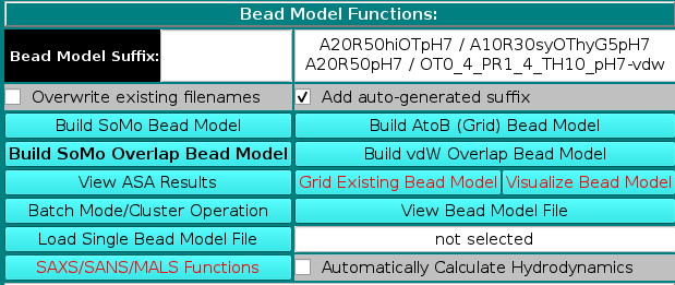
In the Bead Model suffix field you can enter a tag that will be added to the bead model filename, which is automatically generated from the PDB filename by adding "_1" and the extension ".bead_model".
In addition, the Add auto-generated suffix checkbox is selected by default (it can be deselected), and the corresponding field above is populated with a series of alphanumeric characters specifying the main options chosen during bead models generation. These characters will be also added to the bead model filename, to allow for a quick identification of the options used in its generation. Thus, "A20" stands for a residues' ASA cutoff threshold of 20 Å (default), "R50" stands for a bead's ASA re-check cutoff threshold of 50% of its total surface area (default) (see here), "hi" signifies hierarchical overlap reduction in all stages (alternatively, "sy" stands for synchronous overlap reduction), and "OT" means that the outward translation option during overlap removal of exposed side-chain beads is active (see here and here).
The "-so" suffix is added if the Build SoMo Bead Model button is then pressed, while the "-a2b" suffix is instead added if the Build AtoB (Grid) Bead Model button is pressed. In this case, the suffix symbols also include "Gn" for the grid resolution, with n the actual value, and "hy" if the atomic-level hydration option is active (see here). If the Build SoMo Overlap Bead Model is chosen, only the residues' and beads' recheck ASA cut-offs ("A" and "R" values) will be added, with extension "-so_ovlp". If the Build vdW Overlap Bead Model is chosen, suffixes will start with "OTx_y", where "x_y" reports the OT multiplier if different from 0 (see here), and then they will include the ASA probe radius used to identify exposed atoms to be hydrated ("PR#_#, with #_# the radius value in Å) and the threshold accessible surface area thus computed for each hydratable atom ("TH#", with "#" the value in Å2) (see here). The extension will be "-vdw" and no other bead-generation methods symbols will be added, since they have no meaning in this case. However, if the GRPY hydrodynamic computations method is then utilized, and if the Exclude checkbox is selected for the "Inclusion of Buried Beads in the Hydrodynamic Calculations (For GRPY)" option in the Hydrodynamic Calculations Options panel, the "R#" suffix (beads' ASA % re-check cutoff threshold) and a "PR#_#" suffix (ASA probe radius size, Å) will be added with the used values (see here). Finally, the last entry in the suffix field reports the pH at which the model was generated (the pH affects the hydration values at the atomic level).
Upon loading a PDB file and if the Add auto-generated suffix checkbox is not de-selected, the corresponding field will show the four current strings available for SoMo without overlaps, AtoB, SoMo with overlaps, and vdW with overlaps bead models. If any of the options coded in the strings are changed, the field will be automatically updated. The final string will appear once a bead model generation operation is launched. Note that you can keep processing a loaded PDB file after changing any of the various model-building options (see below). If the Overwrite existing filenames checkbox is selected, existing filenames will be overwritten without a warning. Otherwise, a pop up menu will instead appear offering alternative options (see here). The Overwrite existing filenames checkbox is automatically selected for batch mode operations.
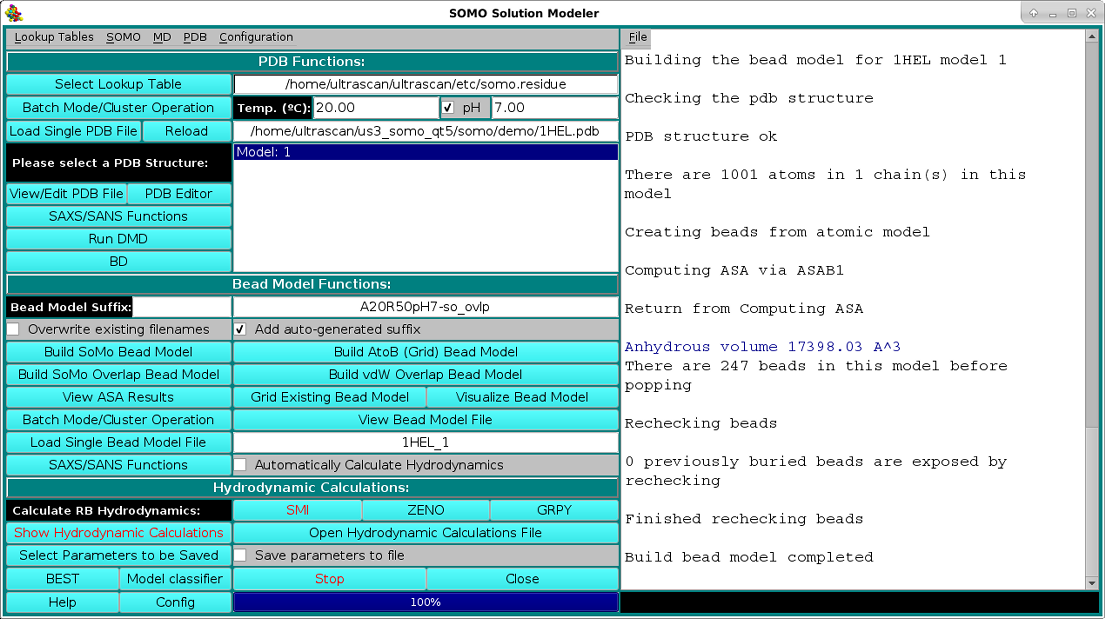
The bead model generation progress of the loaded 1HEL.PDB file using the Build SoMo Overlap Bead Model is shown in the image below:
 |
A fifth button, Grid Existing Bead Model, will operate the AtoB grid routine on a previously generated bead model. This button is not available until a PDB file has been processed with any of the bead modeling primary options (see above), or until a previously-generated bead model file has been loaded (see below). If this operation is launched, the "-a2bg" suffix is automatically added to the filename of the new bead model.
Since model building can take some time, depending on the settings and especially for large structures, selecting the Automatic Calculate Hydrodynamics checkbox will allow the direct computation of the hydrodynamic parameters as soon as the model(s) generation has been completed (the default method is ZENO, but it is user-selectable in the Miscellaneous Options module.). If this checkbox is not selected (default option), at the end of the model building phase the progress bar will be at 100% and the bead model(s) can be visualized with RasMol by clicking on Visualize Bead Model (recommended, comparing the original structure with the bead model could reveal previously unforeseen problems; Warning: if multiple models have been generated, such as from an NMR-style file, pressing Visualize Bead Model will open multiple RasMol windows, one for each model!).
The results of the accessible surface area (ASA) computations (see below) can also be visualized in a pop-up window by clicking on the View ASA Results button; this file also includes the computation of the radius of gyration (Rg) directly from the atomic coordinates of the structure. A just-generated or previously-generated bead model file can also be opened inside a text editor by pressing the View Bead Model File button.
Alternatively, you can load one or multiple previously-generated bead model by clicking on either the Batch Mode/Cluster Operation (see here) or the Load Bead Model File buttons from the menu. In these cases, and if the model(s) was (were) generated/saved in the US-SOMO format, the various settings/parameters used in model generation will be displayed in the right-side progress window. Note that you can decrease the number of beads used, and thus the resolution of the model, by applying a grid procedure on a previously-generated bead model with the Grid Existing Bead Model option (see above). This could be useful when large structures are analyzed, although using the improved AtoB routine on the original PDB file while increasing the grid size (Build AtoB (Grid) Bead Model) seems to produce much better results. By selecting different file types extensions, other type of bead models can also be loaded, like the old BEAMS-format models, or DAMMIN/DAMMIF-generated models. In this case, a pop-up panel appears requesting entering the partial specific volume and molecular weight of the model. The SAXS/SANS Functions button present in this subpanel will allow to perform SAXS-or SANS-related simulations directly on the currently loaded bead model. (see here).
 |
Hydrodynamic Calculations:
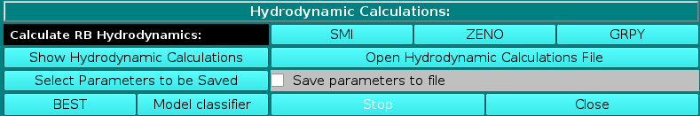
The hydrodynamic parameters can then be determined in the rigid-body (RB) approximation by clicking on either ot the three options present under the Calculate RB Hydrodynamics field: SMI, ZENO, or GRPY. If the bead model was generated by pressing the Build SoMo Overlap Bead Model or the Build vdW Overlap Bead Model buttons, or if it was uploaded and contains either the "-so_ovlp" of the "-vdw" suffix, only the ZENO or GRPY buttons will be available. If the Calculate RB Hydrodynamics SMI button is pressed, the SMI method will anyway perform an overlap test, using the cut-off present either in the bead model file, or that present in the Overlap Reduction Options modules (see here and here), or, if it has been selected, the manual value selected in the Hydrodynamic Calculations Options module (see here). The test will stop after up to 20 overlap instances exceeding the cut-off has been found, listed in the progress window with a message alerting the user that proper action should be taken, like changing the cut-off (not recommended if they substantially exceed the default limits), remove the overlaps, or use the ZENO or GRPY methods. The messages printed in the progress window for the ZENO processing of the SoMo Overlap Bead Model for the 1HEL.PDB structure are shown in the image below, followed by a list of References that should be cited if the US-SOMO-computed parameters are reported in a publication (the list is specific for any particular bead-generation/hydrodynamic computation methods used):
 |
A partial list of parameters can be seen in a pop-up window as soon as the calculations are completed by clicking on Show Hydrodynamic Calculations. The pop-up window will also list the solvent type, temperature and its associated density and viscosity, as set in the Hydrodynamic Calculations options module. A full list of all the parameters is also available as a text file, which can be opened from the results' pop-up window. Such a list from a previously analyzed model can be opened also from the Open Hydrodynamic Calculations File button.
Warning: starting from the February 2021 release, SMI calculations will not report anymore values for the rotational diffusion parameters (like the Relaxation time tau(h)) and the intrinsic viscosity. Recent tests (2020; see the introductory history at the beginning of this Help section) have revealed that SMI calculations are not reliable for the rotational diffusion and intrinsic viscosity calculations. Users can get accurate values for these parameters by running GRPY or, for the intrinsic viscosity alone, ZENO.
The Select Parameters to be Saved button will open a pop-up window (see here) where characterizing/computed parameters can be selected for saving in a comma-separated file for easy import into spreadsheets. Selecting the Save parameters to file checkbox will generate such file, with extension .csv.
The BEST button will open a pop-up window where the hydrodynamic computations results retrieved from a supercompute cluster run using BEST can be analyzed, as shown here.
Finally, by pressing the Model classifier button, you will access a tool for selecting a best matching model among a series of models, by comparing their calculated hydrodynamic parameters with user-provided experimental values (see here).
 |
The black-background bar at the bottom of the progress window will instead report the detailed advancement of some of the steps in the various phases, like the current slice and atoms (or beads) involved in the ASA routine, the iterations in the SMI method, the stage of the LAPACK routines for GRPY. For small structures using the SMI method, or for low number of MC iterations in the ZENO method, these numbers will be barely flashing by in the box, but for GRPY or for large structures using the other two methods they will allow a more in depth monitoring of the various stages. An estimated of the % progress in the hydrodynamic computations for all methods is instead presented and constantly updated as a blue segmented bar with a numerical value in the white-background space at the bottom of the commands side (in the image above, this indicator is shown at 100%).
Operations can be halted at any moment by clicking on the Stop button. To avoid inadvertendly losing data, the Close button will not immediately close US-SOMO, but confirmation will be required in a pop-up window.
Five pull-down menus are presently available to access the various US-SOMO options:
Lookup Tables
SOMO
MD
PDB
Configuration
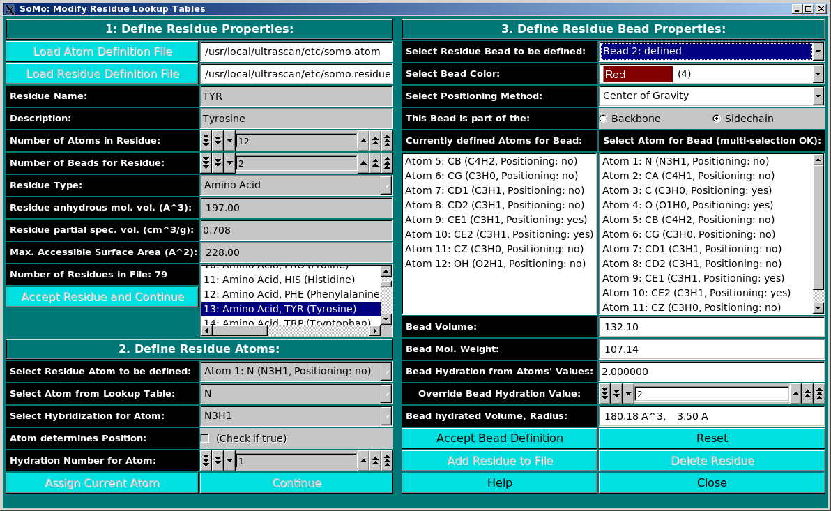
Lookup Tables:
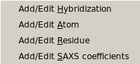 |
From this pull-down menu, you can call four different sub-menus controlling
the four tables containing the definitions of the atoms and residues found in
PDB files, and their SAXS coefficients.
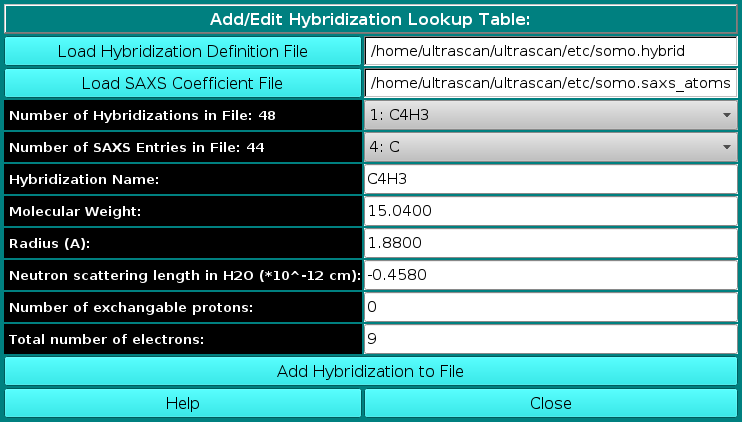
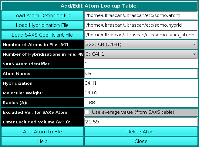
More in detail, you can define/edit the hybridizations, atoms and residues
that need to be interpreted as beads in the bead model generation.
These parameters are collected in different tables that are used
as the components from which the bead sizes and positions are calculated.
PDB structures can then be converted to bead models based on the bead
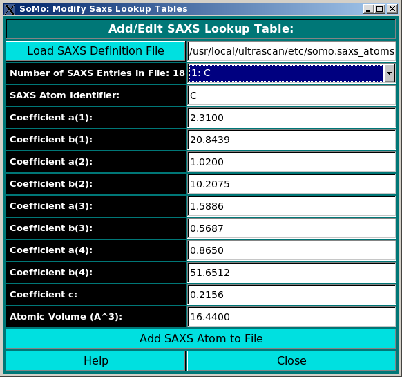
parameters defined here. For SAXS simulations you also need the atomic
scattering factors coefficients (four or five exponentials plus a constant) and the
associated excluded volumes.
SOMO:
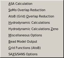 |
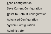
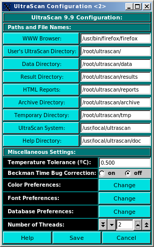
From this pull-down menu, you can access various panels where you can set all the available options for different steps in the program. These options are saved in a system wide config file
$ULTRASCAN/etc/somo.configEvery time you close the SOMO program, the currently defined options will be saved in
$HOME/ultrascan/etc/somo.configwhere they will be reloaded from upon startup.
MD:
 |
PDB Options:
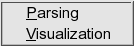 |
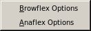
From this pull-down menu, you can access two panels controlling the options for parsing the PDB file and for the model(s) visualization by RasMol.
Configurations:
 |
This document is part of the UltraScan Software Documentation
distribution.
Copyright © notice.
The latest version of this document can always be found at:
Last modified on June 16, 2024.